Document Image Analysis

date:May 20, 2010

Source material for Chapter 18 in Mathematical morphology: from theory to applications

This page describes how to run the applications and generate the figures for the Document Image Analysis chapter in Mathematical morphology: from theory to applications, edited by Laurent Najman and Hugues Talbot, ISTE-Wiley, 2010, The programs for doing this are in the open source Leptonica library.

For reference, here is a version of the chapter that includes the figures. The figures are generated by six programs:

1. livre_makefigs.c This runs the other six programs to generate all the figures.

2. livre_seedgen.c This performs the first step in an approach to page segmentation that identifies image regions by growing a seed into a mask. This generates the seed image for the image regions, which is Figure 1 in the chapter.

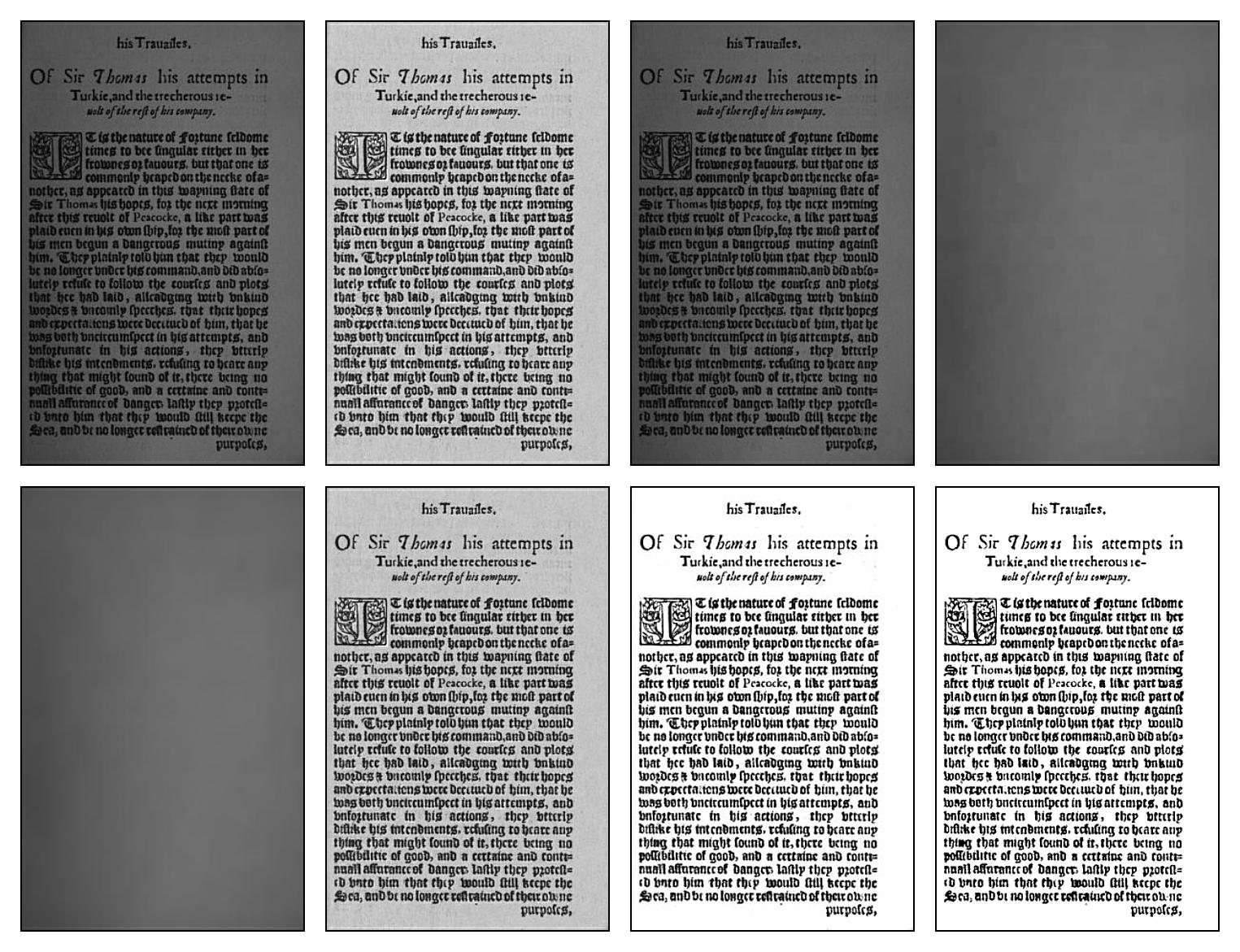
3. livre_pageseg.c This performs page segmentation, showing intermediate steps to identify the text and image regions. It uses a fairly complicated page image as input. It generates Figures 2–5.

4. livre_orient.c This generates Figure 6, a visual representation of the hit-miss Sels that are used for identifying the orientation of roman text, using a statistical count of ascenders and descenders.

5. livre_hmt.c This generates Figures 7 and 8, which are hit-miss Sels that are built automatically from a 1 bpp (bit/pixel) image pattern. Figures 7 and 8 were printed in grayscale. They are reproduced below in color.

6. livre_tophat.c This generates Figure 9, which shows how the tophat operation can be used to normalize and whiten the background of an image with uneven illumination.

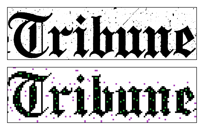
Figure 7

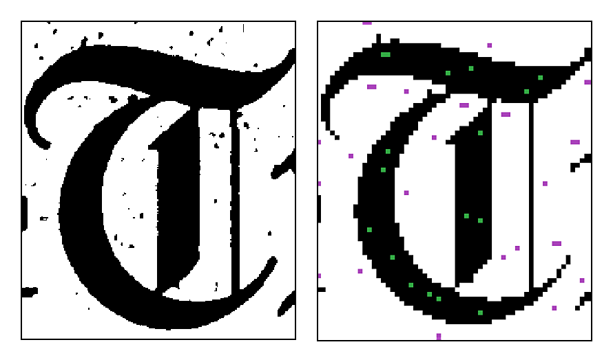
Figure 8

Extra Figure

Additionally, we give a program that generates a figure that was cut from the original paper due to length restrictions. The program, livre_adapt.c, like the tophat, compensates for nonuniform background, but in a more complicated way, by first measuring the background and then doing a locally-adaptive linear mapping in the attempt to make the background uniform. The figure demonstrates a number of operations for doing this. The eight panels are as follows:

1. The input image.

2. The background-normalized color image, where target background value is 200.

3. The input image, converted to grayscale.

4. The grayscale image closed with a 25 x 25 Sel to remove the dark text.

5. The background further smoothed by a convolution, using a 15 x 15 flat-topped block Sel.

6. The background-normalized grayscale image (again, with the target value of 200), using (3) as the input. The result in this case is very similar to (2).

7. Applying a linear TRC (tone reproduction curve) to (6), with the dark point at 30 and the white point at 180.

8. Thresholding the result to 1 bpp.

The most simple way to build these programs and generate the figures is as follows:

• Get the source code from here.

• In the src directory, type make to build the Leptonica library.

• All the programs are in the prog directory. In the prog directory, first type make.

• Then, still in the prog directory, run livre_makefigs. The figures will be placed in /tmp/, named dia_fig1.png, dia_fig2.png, etc.

The leptonica source code can also be found at code.google.com/p/leptonica. To learn about the Leptonica image processing library, read the documentation that starts here.