Color Quantization

date:Sept 4, 2008

How did the need for color quantization arise?

In the old days when computers were slow and memory was expensive, it was difficult to display color images. One couldn’t simply put 24 MB for frame buffers on a video display card. To display color, rather than using 24 bits — 8 bits for each of Red, Green and Blue — per pixel, each pixel was typically only 8 bits deep. These 8 bits then used as an index into a palette, or color table. The color table was in fact a set of three tables, one for each color. Then, using the R, G and B tables in the color table, a single 8-bit index could be used to specify up to 256 different 24-bit colors.

What are the basic problems in color quantization?

Some interesting problems arise. Of the possible 16 million colors that can be described by 24-bit RGB, how do you choose a mere 256 to be the representatives in the color table? How do you display these 256 colors to eliminate visual artifacts from such a small number of colors? And once you have the color table, how do you quickly do the inverse process of finding the best index for each RGB pixel in the image?

The first problem, that of choosing a good set of approximate representatives from a distribution of instances in a much larger set, is an example of vector quantization (VQ). Each of the representatives is a “vector” with Red, Green and Blue components. Each representative will be used as an approximation to the color of some number of actual pixels, and the set of representatives is typically chosen to minimize some error criterion for the actual distribution of colors in the image. The solution of the first problem is represented as a color table for the image.

VQ differs from scalar quantization in that for the latter, the quantization would be an outer product of separate scalar quantizations in each of the three colors. VQ is better because it allows far more flexibility in the way the full color space can be divided up.

Once the color table is selected, the image must be scanned and all pixels assigned an index in the color table. This requires an inverse color map. One brute force approach, by which the 24 bits of RGB are used as an index into a table with 16 million 8-bit indices, requires too much memory. Likewise, another brute force method where for each pixel, the distance to each of the 256 representatives is computed and the smallest is chosen, is impractical because it requires too much computation.

The inverse color map must be performed efficiently. We provide two methods of color quantization, both of which yield efficient (in space and computation) methods for generating the colormap index from the RGB pixel value. The first is a subdivision of the color space into arbitrary rectangles; the second is the octree. Both can be implemented in a way that gives very good results.

Why is error diffusion dithering important?

However, even with the best set of 256 colors, there are many images that look bad. They have visible contouring in regions where the color changes slowly. Flesh colors can be notably poor. The best solution to this problem is error diffusion dithering (EDD), which has the interesting aspect that it typically increases the mean square error. EDD works by computing the error between the pixel value and its nearest representative, and then propagating that error to nearby pixels that have not yet been assigned to a color in the color map. After using EDD, the average color in a small region is very close to the average color in the original, but the individual colors are constrained to be taken from the set defined by the color map. By propagating the error in order to achieve visual color accuracy, EDD thus trades spatial resolution for resolution in depth. Using EDD, a surprisingly bad color quantization can be made to look remarkably good. The point is not that it is OK to do a lousy job of color quantization; rather, if you use dithering, it is not necessary to do an optimal quantization.

There is another interaction between EDD and the inverse color map. Without EDD, the inverse color map needs only be defined for those RGB values that are found in the initial full color RGB image. However, with EDD, the RGB values can be anywhere in the color space, and thus the inverse color map procedure must find a good indexed color for any RGB value.

Finally, for EDD to accurately represent every color, it is necessary that the actual colors fall within the convex hull of the representative colors in the color table. That way, each color can be interpolated between the limited set of colors in the color table. To take an extreme example, if all of the representative colors have a Blue value of 0, it would be impossible to represent any amount of blue in any pixel. In practice, the convex hull criterion is not strictly possible. However, it is important that the representative colors span the color space so that this condition is approximately satisfied.

What methods have been proposed for color quantization?

Going back to the problem of finding a good set of colors, several methods have been proposed. The simplest is a fixed color partitioning, such as one that uses equal volumes of color space. This has the virtue that it can cover the entire color space and does not require a first pass over the image to generate the partitioning. We have implemented a one-pass quantizer, using equal volumes, where each quantized volume is composed of two octcubes that are 32/256 of the color space in each dimension. Using the center of the volume as the representative color, the maximum errors in the (red,green,blue) values are (16,16,32). Partitioning by octcubes is a way of minimizing the maximum pixel error.

Of course, a partitioning that is adapted to use the statistics of the pixel colors in an image will do a better job. This requires two passes, although the first pass, which gathers statistics, need not sample every pixel in the image. There are three types of such adaptive color quantizations for which practical implementations have been made: popularity, median cut and octree. The division of the color space can be represented by a tree, and this tree can be generated either by starting with the entire color space and splitting it up, or by starting with a large number of small volumes and merging them. The division of colors along a line can be either flat or hierarchical. The popularity method uses a simple selection of colors from the color space, the median cut method uses a splitting algorithm designed to have roughly equal number of pixels in the resulting rectangular volumes, and the octree method is hierarchical and is naturally amenable to an algorithm that merges (as well as splits) regions of color space.

Before we discuss these, I should mention that there is another type of clustering, called K-means, along with related vector quantization methods such as the Linde-Buzo-Gray algorithm for clustering for data compression. In K-means, you start with an initial set of centers, make a pass over the image to assign each pixel to its nearest center, compute the centroids of each cluster so obtained, and use these centroids as the centers for the next iteration. The total error is guaranteed not to increase from one iteration to the next, so the method will converge to a locally optimal solution. However, it is not guaranteed to be globally optimal; the final centers will depend on the initial centers that are chosen. The LBG algorithm is similar. These clustering methods are not practical for color quantization because, in addition to sensitivity to initial conditions, they require many iterations and are very slow.

The popularity method selects the color representatives from the set of most popular colors. Make a histogram of the actual colors in an image (say, clipped to 15 bits so that you have a significant number of pixels in the most popular colors), and choose the top 256, for example. This method does poorly for images that have many different colors represented. For example, if the image has a small number of pixels of some particular colors, these colors will not be represented at all. It also does poorly when using dithering (see below) because dithering can only interpolate within the convex hull of the representatives. Consequently, we have not implemented this.

The median cut method attempts to put roughly equal numbers of pixels in each color cell. It is implemented by repeatedly dividing the space in planes perpendicular to one of the color axes. The plane can be chosen to divide the largest side and to leave about half the pixels in each of the resulting regions. This method does well for pixels in a high density region in color space, where both the cell volume and color error is very small, but the volume of a cell in a low density part of the color space can be very large, resulting in large color errors.

In the open source jpeg library implementation, half the representatives are chosen by the median cut, and half are chosen by dividing up the volume in the largest remaining regions. This reduces the largest color errors that may occur, and spreads the representative colors out more evenly through the color space. The latter allows better results with dithering.

Octrees are another good way to divide up the color space, while allowing fast indexing for an inverse color table. One method has been published, by M. Gervautz and W. Purgathofer, a summary of which can be found in Glassner’s Graphics Gems I, 1990. This method builds an octree by taking pixels, one at a time, and either making a new color or merging them with an existing color. After the prescribed number of colors in the color table have been established, the new pixel either makes a new color (causing merging of two existing colors), or it is merged with an existing color. Each color is represented by an octcube, or set of octcubes, so the merging operation effectively prunes the (potential) octree. This method has the advantage that only up to 256 colors need be stored at any time. It has the disadvantage that the merging operations are complicated, and it is not easy to understand how to represent the full color space, which is necessary for dithering. In fact, the description was so sketchy that I can only commend D. Clark for providing an implementation in Dr. Dobb’s Journal (reference at the end of this section).

Leptonica provides two methods of color quantization: Modified Median Cut Quantization (MMCQ) and octree quantization (OQ). Both can be designed to be fast, to give reasonably good results without dithering, and to give very satisfactory results with dithering.

In MMCQ, as in the median cut method, the color space is divided up into a set of 3D rectangular regions (called “vboxes”). These are derived by splitting from a large vbox that contains all the original pixels in the image. Further, if dithering is allowed, the original vbox must be the entire RGB space, to assure that any possible RGB value is in one of the final subdivided vboxes. Quantization of color space is to a fixed level, given by the number of bits that are retained for each component. We call the smallest possible vbox the “quantum volume.” Typically, when using a colormap of 256 colors or less, 5 bits are sufficent for each component, so there are 2¹⁵ of these quantum volumes filling the entire color space. With respect to the 8 bit/component quantization of the original RGB image, each quantum volume is then a cube holding 2⁹ = 512 of the original 2²⁴ colors. The smallest vbox is one quantum volume. Because there are 2¹⁵ of them in the color space, on average, each vbox has 64 quantum volumes. For a typical image, the highly populated vboxes will be relatively small, and, as we will see, the largest vboxes will be nearly unoccupied.

In adaptive (2-pass) OQ, the entire color space is represented by the root octcube. The octcubes at each level are further subdivided, depending on occupancy. This is somewhat more difficult to visualize than MMCQ. It is described in more detail below, and in the code in colorquant1.c.

Modified median cut implementation

In colorquant2.c, we’ve implemented a modified version of Paul Heckbert’s median cut algorithm, which he published in Color Image Quantization for Frame Buffer Display, in Proc. SIGGRAPH ‘82, Boston, July 1982, pp. 297-307.

The Heckbert “Median Cut” algorithm says to repeatedly divide 3D regions in colorspace in such a way that the two parts have roughly equal number of pixels. Heckbert also suggests choosing the axis for subdivision based either on the length of the side or the variance of pixel values along that axis. The implementation starts with a computation of the histogram in quantum volumes, which is typically an array of size 2¹⁵. This is used to determine which vboxes to split and where to split them. After all splitting is done, the colormap is assigned, with one color for each vbox, and the histogram is converted to an inverse colormap containing the colormap index for each quantized rgb value. Finally, the inverse colormap is used to generate the quantized image. This is conceptually very simple.

A number of important implementation decisions are not discussed. Consequently, different “implementations” of “median cut” will significantly vary in the quality of the quantization, depending on the pixel distribution in color space and the details of the implementation. This is important to keep in mind when you are told how well an algorithm performs: the algorithm has to be sufficiently specified so that it can be constructed in a unique way from the specification.

Heckbert’s paper was written in 1982. Today, with open source, an algorithm can be fully specified with the code itself. I found that implementing median cut was a very interesting exercise. First, doing an implementation brings up various decisions that must be made. Second, I found that median cut doesn’t work well on images, such as paintings, that have small amounts of spot color that need to be in the colormap. The flaws in the method then led to an understanding of the requirements for a successful approach to quantization.

One immediately sees that there are three main decisions outside of the original description that must be made.

1. How do we schedule the existing set of vboxes for further subdivision?

2. How do we decide the axis along which to divide the vbox?

3. When dividing the vbox along the chosen axis, in which part do we put the bucket containing the median pixel?

Following one of Heckbert’s suggestions, I chose the axis to be the largest dimension of the vbox. For the third question, suppose we represent each component in color space by 5 bits. Then the maximum length in quantized units of a vbox is 32. Suppose we have a vbox where the maximum length is N. Choose that direction, and build a histogram of the number of pixels falling inside each of the N buckets, by summing over the region in the other two directions. Suppose the median pixel falls into the Mth bucket, where buckets are numbered from 0 to N - 1. Then there are M buckets to the “left” of the Mth bucket, and N - M - 1 buckets to the “right”. When you subdivide, put the Mth bucket into the smaller of the “left” and “right” parts. This has the effect of making the two parts closer in size, because the partition line is moved into the larger of the parts. For the first question, the obvious choices are using a simple queue and using a priority queue based on total occupancy. The priority queue is preferable for several reasons, one of which is that it does a much better job of breaking up the high occupancy regions so that they are as close to equal population as possible. The effect on image quality is that washes composed of many pixels with slow spatial color variation are well-quantized to avoid posterization.

But even if you make all these choices, you will find that small color clusters will not be represented in the color map. The reason is that any small cluster that is included in a vbox with a large cluster (that is not so big that it is further subdivided) will be represented by a colormap color determined by the large cluster. For these situations, median cut does poorly.

However, a simple modification of median cut does a much better job representing the small clusters. We want to cleanly separate the small clusters from the larger ones. To do this, move the partition line even farther into the larger side (“left” or “right”). Surprisingly, the best results appear to happen when we place the partition line not near the median pixel, but in the center of the larger of the two blocks (“left” and “right”) on either side of it!. What is happening? By putting the cut line far from the dominant cluster, we give the small cluster a chance to be properly represented in the colormap. And because we are using a priority queue, it doesn’t matter that the larger cluster wasn’t partitioned: it will come right back to near the head of the queue for further subdivision. Higher density clusters will be repeatedly subdivided into smaller regions, and the modification only applies when the larger of the “left” and “right” blocks is 2 or more. This modification is part of the reason I’m calling the algorithm MMCQ — we’re not really splitting close to the median.

But we’re not finished with necessary modifications. There are still flaws in the result. If we choose all partitioning based on population, there may be very large vboxes with considerable population that are not split. Without dither, these can appear as large posterized regions; with dither, serious artifacts can develop, where the error is significant and the accumulated error manifests itself periodically in pixels of very different color. This situation must be avoided.

The dither oscillations can easily be prevented by putting an upper bound on the amount of error that is propagated to neighboring pixels. It is reasonable to do this for safety. But a more general improvement is needed, that will split regions that are large with a significant population, but may not have enough pixels to get to the head of the queue. The jpeg quantizer uses population to schedule half the splits and vbox size for the other half. Here’s what we do:

1. Generate a fraction f of the requested output colors by splitting vboxes based on the number of pixels in the box.

2. Then generate the remaining fraction (1 - f) of colors by splitting based on the product of the population times the volume of the vbox. If we were to use simply the volume, we would waste colors by splitting vboxes that have no pixels.

We need a nonzero value of f because it is important to balance the splitting of the most populous vboxes with the splitting of the largest well-occupied vboxes. It turns out that the result is not strongly dependent on the fraction f, and very good results can be obtained for f between 0.3 and 0.9. The independence of the quantization quality with respect to f is encouraging, because it indicates that good results can be generally obtained with a single choice of this parameter.

Overall, the undithered MMCQ gives comparable results to the Two-pass Octcube Quantizer (OQ). Comparing the two methods on the test24.jpg painting, we see:

• For rendering spot color (the various reds and pinks in the image), MMCQ is not quite as good as OQ.

• For rendering majority color regions, MMCQ does a better job of avoiding posterization. That is, it does better dividing the color space up in the most heavily populated regions.

After splitting the colorspace, we generate a pix colormap by representing the color in each vbox by the average color of the pixels there. (If there are no pixels, we use the center of the vbox.) At this point we no longer need to keep the histogram of pixels in each quantum volume, so we turn the histogram into an inverse colormap, where every quantum volume in a vbox is labelled by the colormap index representing the vbox. The final step in quantization is to compute, for each image pixel, the value of the colormap index to use. The inverse colormap allows this to be done with a simple table lookup. If we are dithering, there is some added computation to propagate the error to pixels that have not yet been indexed.

For a summary of our modified median cut quantization algorithm, I’ve written a report.

Octree implementation

What is the octree data structure used in Leptonica?

The method we use in Leptonica is fairly simple, both conceptually and in implementation. Our basic data structure is a pyramid of arrays, describing the leaves of an octree at each of the levels 0 through 4 (or 5 or 6). At each level, there are 8 cubes that correspond to a single cube at the level above. The cubes are indexed so that the cube i at level l contains the eight cubes 8i+j, j = 0, ... 7 at level l+1. The cube index is computed from the RGB values by taking the most significant bits of the three samples in order:

r7 g7 b7 r6 g6 b6 r5 g5 b5 r4 g4 b4 r3 g3 b3 ...

down to the level of interest. For example, at level 5, the index consists of the 15 bits that are shown above. For any RGB value, it is easy to compute the cube indices at any level of the octree, and we provide lookup tables to make this fast. Note that the octree that is represented by this set of arrays is virtual, given by the indexing relation above, because there are no pointers going between different levels! We just have arrays of these cube data structures, with fast indexing into the arrays. Keep this “pyramid” in mind in the following description of the algorithm

How is the octree formed?

There are two passes. The octree with the selected color table entries (CTEs) is built in the first pass. To build this, we only need to label the specific octcubes within these arrays that are to represent the CTEs; we do not need to build any other data structures. How do we determine which cubes to label? In the first pass, we place the pixels in octcube leaves at a designated depth or level, which can be 4, 5 or 6. With level 5, there are 2¹⁵ = 32K leaves. We store only the number of pixels in each of these leaves. The tree is then pruned in the following way. Starting at the deepest level, and iterating for every cube at that level, check the octcubes in sets of eight, where the eight octcubes are those that compose the octcube at the next level up. For each set of eight octcubes, one of the following will pertain:

1. One or more of the cubes has enough pixels to become a CTE. Make it a new CTE.

2. One or more of the cubes has already been selected as a CTE.

3. None of the cubes is already a CTE or has enough pixels to become a CTE.

In both the first and second cases, the octcube at the next level up automatically becomes a CTE, which contains those pixels that are not in a subcube that already is a CTE. In the third case, the pixels are simply aggregated into the octcube at the next level up. When all cubes are done at that level, the procedure is repeated at the next level up.

The decision for forming a new CTE is that the number of pixels in the cube exceeds a threshold that is proportional to the number of pixels yet to be assigned to a color divided by the number of colors left to be assigned. We actually hold back 64 colors in reserve, because when we get to the second level we require that each of these 64 octcubes be a CTE by default. In this way, we constrain the maximum color error while insuring that the entire color space is covered by the color table. The value 1.0 for the proportionality constant at each level works well. (The proportionality constants for levels 0, 1 and 2 are not used, because the octcubes at level 2 become CTEs automatically.)

What color is associated with each octcube in the color table?

We associate with each octcube in the color table the coordinates of the center of the cube. This is easier than maintaining a running centroid, and has very little effect on the result. In fact, because the octcubes at each level are indexed as they would appear in the octree from left to right, we can quickly compute the center of the octcube in which any pixel would fall, so we don’t even need to store it.

How are color indices assigned to the image pixels?

The second pass, where the pixels are assigned their index, can be done very quickly in two different ways, of which we implemented the second:

1. Make an explicit inverse colormap. Compute and store the index in the leaf array at the deepest level (in the place where we initially stored the histogram). Then for each pixel, convert the RGB value of the pixel to the truncated octcube index at that level, and look up the colortable index from the pre-computed array.

2. For each pixel, run down the tree from the root to find the octcube that it belongs in. Do this by converting the RGB value to an index into the array of octcubes at each successive level, stopping when you find an octcube that is marked as a CTE and the octcube at the next level down is not a CTE. (If you reach the bottom level, take that octcube.) Then take the colortable index from the CTE octcube. For dithering, you also need to know the center of the octcube, which can either be computed or read from the value stored there.

This octree method has the drawback of not generating exactly the number of colors requested for the color table. It typically has a few less. The actual number depends on the distribution of colors in the image. Note that if enough pixels are present to make a CTE from an octcube at level 6, then CTEs for the containing octcubes will be generated automatically at levels 5, 4, and 3, regardless of the number of unassigned pixels in those cubes. (The only exception is if all 8 subcubes of an octcube are already CTEs, the containing octcube will be labelled as a leaf for purposes of traversing the tree in the labelling step, but will not be assigned a color).

How is the error diffusion dithering applied?

To maximize the accuracy of the color appearance, we use EDD in the second pass. The error in each of the three samples is passed down to three adjacent pixels whose indices have not yet been computed. We use just three pixels, with fractions of 3/8, 3/8 and 1/4, for simplicity. The implementation uses six color buffers for the pixels in the current line and the next line, and does all computation in integers with a multiplying factor of 64 to reduce the roundoff error. To the extent that the actual RGB pixel colors are within the convex hull of the CTE values, EDD will accurately reproduce the original pixel color when averaged over a few pixels.

How fast is the implementation?

For efficiency, the first pass, where the octree color table is generated, can be done on a subsampled version of the input image. For an image with a million pixels, subsampling by 4x in each direction is perfectly adequate, as it leaves about 70K pixels to form the octree. The conversion speed for generating a colormapped image from an RGB image depends on the deepest level at which pixels are allowed to form CTE octcubes. On a million pixel RGB image, using a 3 GHz Pentium, the total conversion time in seconds is:

Timings for Image Generation using Octree Color Tables

	octree levels
	4	5	6
no dither	0.03	0.04	0.08
dither	0.08	0.09	0.13

All details are found in the code in colorquant1.c and colorquant.h, where you will find 8 different implementations. The two-pass adaptive method gives the best results (in fact, typically a little better than the median cut). However, other octcube-based implementations are useful for specific types of images. For example, map images with a relatively small number of well-populated colors, but having a large number of different colors due to anti-aliasing, are quantized well using pixOctreeQuantByPopulation(). See the regression test, prog/colorquant_reg.c for usage and results on a number of different images. It should be emphasized that when using error diffusion dithering, you get a reasonable job of visually representing the color, even for simple, non-adaptive methods of quantization. However, without EDD, non-adaptive methods look poor on most images. In the examples below, pixFixedOctcubeQuant256() is used for one-pass quantization, and pixOctreeColorQuant() is used for two-pass quantization.

For more information on octree color quantization, I’ve written a report. There are five comparative images referenced in the report. These are given below. It should be noted that the actual rendering of these images will depend on the browser, the frame buffer depth (8, 16 or 24 bits) of the computer, and the video display card.

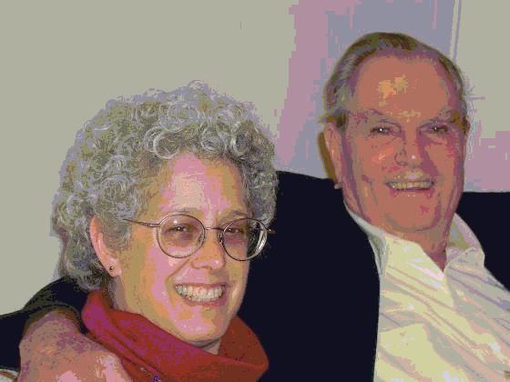
One-pass quantization, no dithering

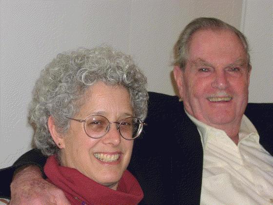
One-pass quantization, with dithering

Two-pass octree quantization, no dithering

Two-pass octree quantization, with dithering

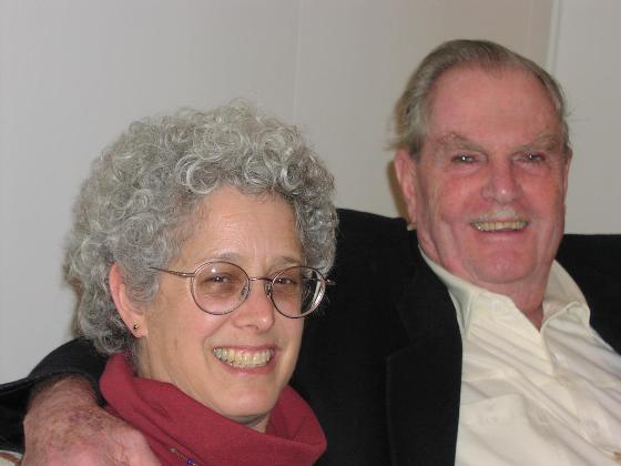
Full RGB color image

For further reading on color quantization . . .

• Color quantization in the wikipedia.

• Paul Heckbert’s original paper. Color image quantization for frame buffer display, Computer Graphics, Vol 16, No. 3, pp. 297-307, 1982.

• The popularity algorithm, D. Clark, Dr. Dobb’s Journal, pp. 121-128, July 1995.

• Median-cut color quantization, A. Kruger, Dr. Dobb’s Journal, pp. 46-54, 91-92, September 1994.

• Color quantization using octrees, D. Clark, Dr. Dobb’s Journal, pp. 52-57, 102-104, January 1996.