Grayscale and Color Image Enhancement

date:Sept 27, 2008

What do we mean by grayscale and color image enhancement?

I’ve put a few operations here that are relatively simple and in wide use for improving the appearance of grayscale and color images. Each one will be described below. The first two, gamma correction and contrast enhancement are trivial to implement because they only require a lookup table to map from the source pixel value to the dest pixel value. The last two, unsharp masking and image smoothing are a little more complicated because they use some set of neighboring pixels in the source to determine the dest pixel value. All four operations work separately on each color sample, so the color implementation for each one just uses its grayscale implementation three times (once for each color sample). There are many other image processing operations that can be included here, and they will be added as occasion permits. If you have a favorite that’s not here, ask me.

What other types of enhancement operations exist?

Image restoration takes an image that has been degraded by some known (typically statistical) process and attempts to regenerate something closer to the original image. These methods are often Bayesian, selecting destination pixels using a maximum a posteriori procedure. The basic idea is very simple. You have a statistical model for the degradation process, given as a set of conditional probabilities for observing a specific degraded pixel when you started with some original pixel. You also have an estimate of the prior probabilities for the original image pixels (or groups of them). Bayes law then lets you estimate the posterior conditional probabilities, which are the probabilities that, given an observed (degraded) pixel, you started with some original one; and you select the maximum of these over the set of all possible original ones. By doing this, you select the original image pixel that is most likely to have produced the observed pixel.

If the noise is known to be sparse additive gaussian (“sparse” meaning that only a small fraction of the pixels are affected), an obvious operation to apply is a median filter, which is very good at removing outliers without seriously affecting other pixels. It is nonlinear, has some smoothing effect, and tends to change pixels at sharp edges.

For binary images, enhancement involves a number of operations, such as removal of pepper noise. If the image has been scanned, cleanup can involve deskew, removal of black pixels near the edge, and special operations on binarized pictorial regions. The latter can involve conversion to gray, followed by grayscale enhancement and halftone screening back to binary. Many scanners give you binary output, and if they threshold the pictorial regions without halftoning or dithering, the result is a high contrast image where much of the gray information can be lost.

If the image is a binary scan that is composed of connected components, many of which are similar (such as text characters), it can be enhanced on a component basis. Use the jbig2 clustering algorithms in Leptonica to put all instances of connected components that are sufficiently similar into the same class. Then from that set of instances, generate a template with less edge noise. This template can be either binary or grayscale; the latter gives an improved appearance because the edge pixels will be gray, causing the edge to appear smoother. Then build the reconstructed (enhanced) image by substituting the template image for each of the instances that were used in deriving it. See the page on the Jbig2 Classifier for more details.

Gamma correction

(The discussion in this section almost certainly contains inaccuracies. I will remove this caveat when I have sufficient confidence in its accuracy.) Cathode ray tubes (CRTs) have a nonlinear response between current from the thermionic tube and applied voltage. Plotted this way, the current has positive curvature with voltage, which corresponds typically to a gamma of about 1./2.2. By this we mean that the output current is proportional to the input voltage raised to the power 2.2. Low voltages have very low currents. Now, because we want the response to be linear, so that what we see on the CRT is the same as the actual image taken with a digital camera, the cameras are calibrated to compensate for the display device by having a gamma of 2.2. All pixels in the captured image are lightened, with dark areas being lightened relatively more. It would be nice if all display devices were calibrated so that they would display images similarly. In a perfect world everyone would follow the same rules, but Apple sets up its CRTs to have a gamma of 2.4.

But things get much more complicated with flat panel displays. Whereas CRTs emit light from the phosphor that is proportional to the electron current hitting it, flat displays use a white illumination with light subtraction due to absorption in the dyes. Flat panels do not have a built-in physical gamma to darken the image; consequently, images look much brighter than on CRTs.

There is also a calibration for displays that has to do with the relative amount of different colors used to produce white. This is expressed by the temperature of the black body radiator that would produce this color distribution. The standard is 6500 degrees K, but manufacturers have found that if they use higher equivalent temperatures, the displays are brighter, and the extra blue is not too noticeable because the eye is relatively insensitive to blue. So, for example, an inexpensive CRT may be calibrated to 12000 degrees K.

What about printing? If you print from a digital camera image without using a gamma correction, the image will appear light and washed out. So printing software typically compensates for the high gamma of the camera.

From a psychophysical viewpoint, people experience intensity logarithmically. Each doubling of the intensity is perceived as an additive constant to the apparent brightness. Our eyes have a dynamic range of about 10⁶, whereas your camera has a mere 8 bits (256 levels) in each color. If the camera were linear, a scene with both light and shadowed regions could have both the shadowed region too dark and the light region washed out. The positive gamma built in to cameras helps somewhat in this respect. The apparent dynamic range in the dark parts of the image is increased, because more of the actual range is assigned to these darker pixels. This gives the camera a logarithmic response. Of course, the lighter part gets even lighter, but not by as much.

So gamma mapping is used both to compensate for nonlinearities in the display devices and to increase the apparent dynamic range. The output is related to the input by raising it to the factor (1 / gamma), properly scaled so that the end points are not adjusted. The mapping function looks like this:

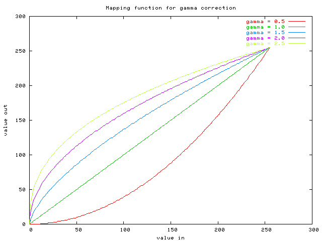
The plot was made using prog/gammatest.c. If gamma < 1.0, the image is darkened, with the biggest effect happening for the dark (low input) pixel values. If gamma > 1.0, the image is brightened overall, with the largest changes happening again for the dark shadows.

We provide a top-level interface pixGammaCorrect() in enhance.c. For display on a CRT, depending on the source of the image, you may want to apply a gamma in the range 1.5 to 2.0. For printing, again depending on the image source, you may want to apply a gamma that is less than 1.0 to darken the image.

Contrast enhancement

To increase the contrast, the pixels above some mid-value are lightened, while those below are darkened. For an image that is washed out, and still has too little contrast after gamma correction to darken, using a gamma < 1.0, the contrast can be increased by applying a sigmoid-shaped mapping function to the input pixels.

How does one generate a sigmoid curve? One obvious way is to integrate under a gaussian; this gives a set of curves with a single parameter. Unfortunately, such an integral is not an elementary function, so you’d have to use a table. As an alternative, consider integrating under a lorentzian. The lorentzian goes as 1/(a² + x²), and consequently has large tails compared to the gaussian. But the lorentzian integrates simply to the arctan function. This makes a transition between -pi/2 and +pi/2 as the angle goes from large negative to large positive values. Using a single parameter to scale the angle, the result is to take a slice of the function centered about 0. The parameter is just the width of the slice, in appropriate units. As the parameter approaches 0, the width gets small, so we’re using the arctan function near 0, which is linear and hence sets the output equal to the input. As the parameter increases, the contrast increases. The output is scaled and translated so that the min and max values of input and output coincide (here, at 0 and 255). The mapping function looks like this:

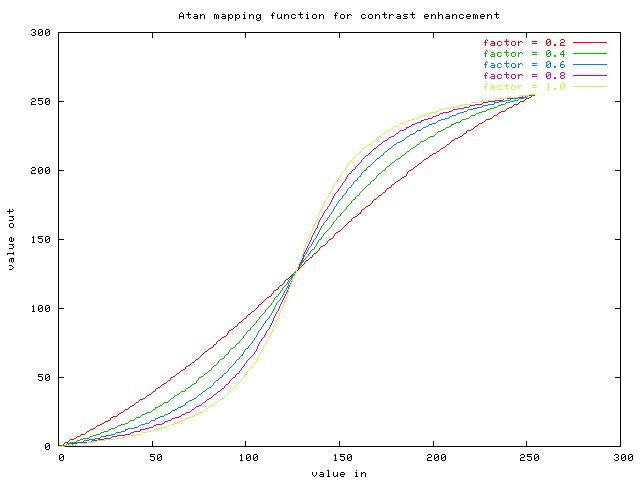
The plot was made using prog/contrasttest.c. See that file or the implementation in pixEnhanceContrastGray() for details. Values of the input parameter greater than 0.0 increase the contrast. (Values less than 0.0 should decrease it; this is not implemented, however.) The top level interface, which takes both 8 bpp grayscale and full color images, is pixEnhanceContrast() in enhance.c.

Unsharp masking (edge enhancement)

When an image has been degraded by blurring, due to a low-pass filter in the optics or subsequent image processing, the pixels most affected are at “edges” where the intensity changes quickly in some particular direction. These edges can be sharpened by running a high-pass filter to emphasize the pixels near edges and then adding some of this back into the image. It should to be done in such a way that the overall intensity of the image is unchanged, and this requires that the high-pass image be shifted downward to have an average pixel value of 0. Then bright edge pixels give values that are added to the original, whereas dark edge pixel values are subtracted.

The method implemented here is called unsharp masking. The high pass “edge” image is generated by convolving the image with an approximation to a laplacian filter. In such a filter, the center has a value 1.0 and some set of N surrounding pixels each has a value -1.0/N. For a 3x3 filter, this would look like:

-1/8   -1/8   -1/8
-1/8     1    -1/8
-1/8   -1/8   -1/8

We implement this 3x3 high-pass filter by first generating a low-pass image using a 3x3 smoothing filter:

1/9    1/9    1/9
1/9    1/9    1/9
1/9    1/9    1/9

and then subtracting it from the original image. The result is:

-1/9   -1/9   -1/9
-1/9    8/9   -1/9
-1/9   -1/9   -1/9

which is identical with the laplacian given above except for an overall scaling factor of 8/9.

Once the edge image has been generated, some fraction of it is added to the original image. Thus, there are two parameters:

1. The size of the smoothing filter, given by 2s + 1. For s = 0, the filter has unit size (support), and hence it is the identity. The edge image is then 0, so there is no edge sharpening. The 3x3 filters given above are used to generate the edge image when s = 1.

2. The fraction f of the edge image added back. Typical useful values of f range between 0.2 and 0.7.

The low-pass image is generated using the block convolution function, which does the convolution in a time independent of the size of the filter. The arithmetic is all done on 16 bit unsigned arrays, with appropriate shifting to represent negative values. Details can be found in pixUnsharpMaskGray() in enhance.c The top level interface, which takes both 8 bpp grayscale and full color images, is pixUnsharpMask().

Image smoothing

I have included this for completeness, as image smoothing is one step in the edge enhancement method described above. This is a low-pass filtering operation. The top level interface, which takes both 8 bpp grayscale and full color images, is pixBlockconv(). The method uses an intermediate accumulation matrix so that the speed is independent of the size of the filter. The filter is restricted to a rectangular kernel of constant (normalized) height.